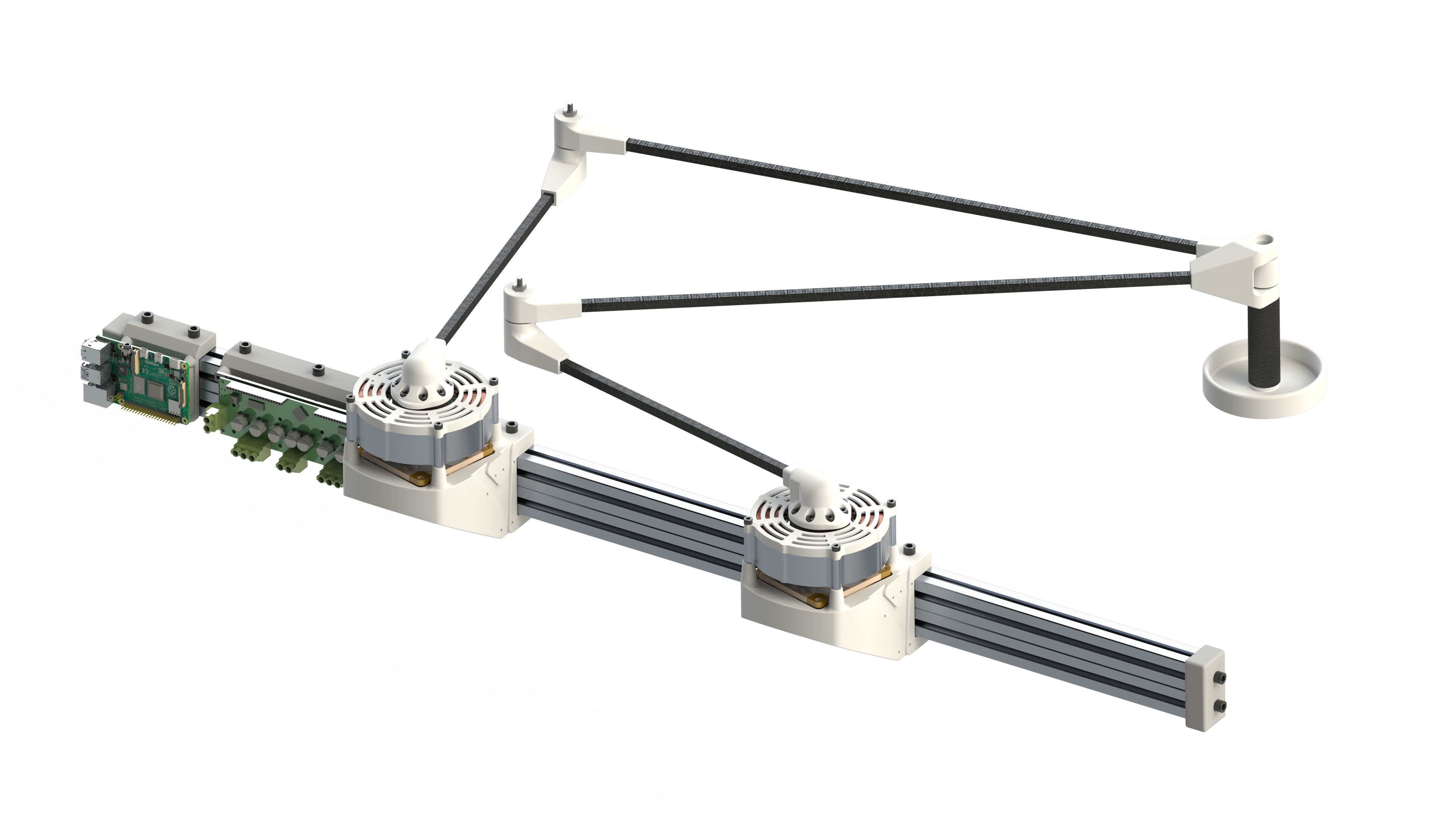
Five-Bar Robotics: Kinematics and Dynamics

For my honors thesis I made a five bar robot that could play air hockey. More on that and the custom hardware required to make that happen in a future post (sneak peek of the render above!), but for now we are going to talk about the kinematics and dynamics of this robot. In this I’ll include a few diagrams and a traces of the robot motion and links to some of the papers and code I used to make this happen.

Forward Kinematics of a Five-Bar

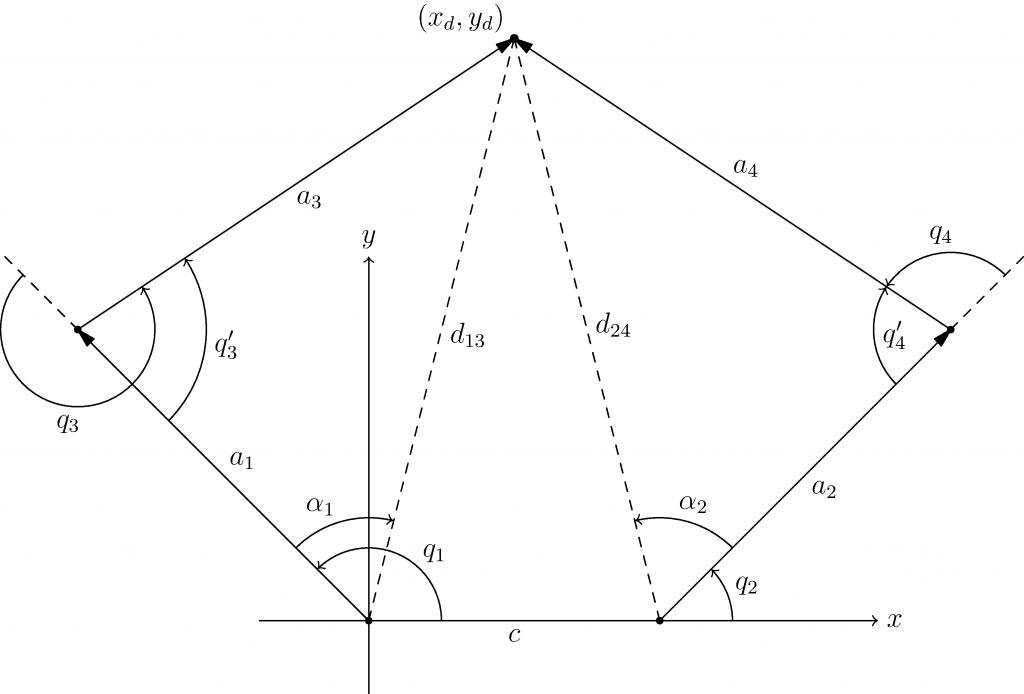
The forward kinematics of the five-bar can be determined using the standard rules of geometry and a healthy portion of cosine and sine. Using the diagram below, it is clear that if we assume joint 1 to be at position $(0, 0)$ , the point $(x_d, y_d)$ would be just be the sum of the x and y components of each side of the five-bar.

A diagram with four moving bars connected to the fifth bar that is the ground. This creates a five-bar mechanism. Each of the angles are labeled such that the end point can be defined. — A diagram with four moving bars connected to the fifth bar that is the ground. This creates a five-bar mechanism. Each of the angles are labeled such that the end point $(x_d, y_d)$ can be defined.

This leaves us with the following equations for the end effector point, finishing the forward kinematic analysis.

Inverse Kinematics of a Five-Bar

Because that was too easy, we now graduate to the inverse kinematics problem. For the five-bar robot this is both surprisingly easy and hard. Because of the redundant nature of the robot, we see that there are four solutions of angles that reach $(x_d, y_d)$ . To envision these other solutions, imagine reflecting the two bars across their respective dashed lines.

The method used here will make use of several facts about the geometry of the system and use the cosine rule. The cosine rule can effectively define $q_3^\prime$ , $q_4^\prime$ , $\alpha_1$ and $\alpha_2$ , so we can then solve for each.

$d_{13} = \left(x_d^2+y_d^2\right)^{1/2}$

$d_{24} = \left(\left(x_d-c\right)^2+y_d^2\right)^{1/2}$

$q_3^\prime=\arccos\left(\frac{d_{13}^2-a_1^2-a_3^2}{2 a_1 a_3}\right)$

$q_4^\prime=\arccos\left(\frac{d_{24}^2-a_2^2-a_4^2}{2 a_2 a_4}\right)$

$\alpha_1=\arccos\left(\frac{d_{13}^2+a_1^2-a_3^2}{2 a_1 d_{13}}\right)$

$\alpha_2=\arccos\left(\frac{d_{24}^2+a_2^2-a_4^2}{2 a_2 d_{24}}\right)$

Using these solutions, we can then solve for $q_1$ and $q_2$ . This creates four total solutions. This can be done as follows:

Each of those represents a possible solution of joint angles that reaches $(x_d, y_d)$ . Given a set of current angles, one of these solutions will likely be the closest and most reasonable solution to move towards. Because of this, the associated code on my GitHub determines the best solution based off your current position in terms of angles.

Five-Bar Robot Dynamics

The code and equations for the dynamics are massive and cumbersome, but can be written in the standard form of differential equations for ridged body systems. If you want to know more about this, check out this paper someone made on this and the code I made to simulate it.

Not only did I make code to simulate the five-bar under a set of initial conditions, I also made code that simulated the five-bar following a given path with a PD controller. I include this here because I thought it was a cool demonstration on how PD gains can affect the speed and accuracy of the tracking for the robot. I also found that the robot, when tuned aggressively, had to follow the path closely or it would go out of control. This indicated to me that some form of gain scheduling based on the distance to the desired path would be needed if this control strategy was used. I have not implemented this feature yet, but it seems like something I should look into.

For each figure, the bar on the left represented the color of the line over time from time=0 seconds to time=10 seconds. The robot gets to the final position before 10 seconds, so you will not see the entire color range. You can see this color change best on the poorly performing PD controller due to the extra settling time.

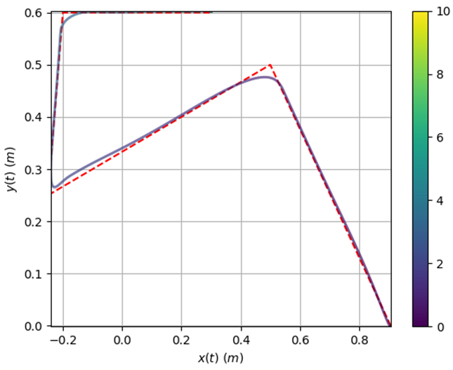
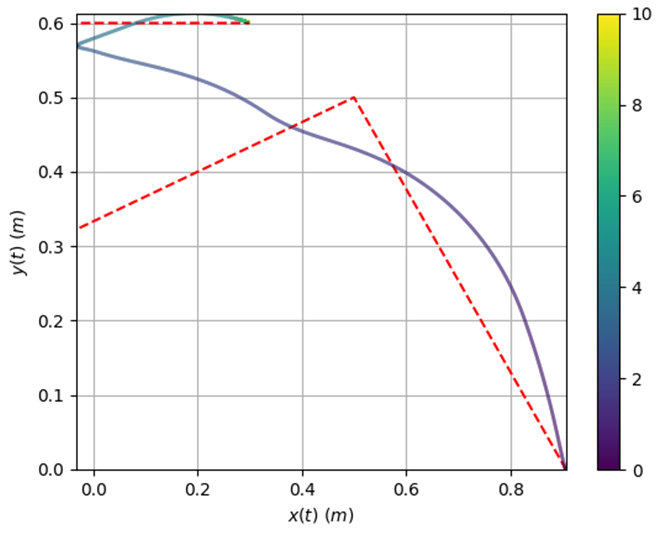
For a medium Kp. (Kp=50 Kd=5) we see that the five-bar robot follows the line pretty well.

For a small Kp. (Kp=5 Kd=5) we see that the five-bar robot follows the line poorly.

On the left we can see that for a medium Kp PD controller (Kp=50 Kd=5) the five-bar robot follows the line well. On the right we can see that for a small Kp PD controller (Kp=5 Kd=5) the five-bar robot does not follow the line effectively.

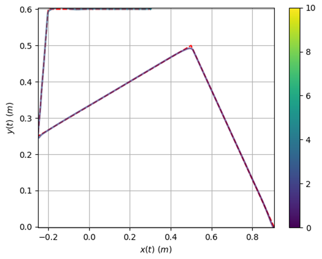
For a large Kp. (Kp=150 Kd=5) we see that the five-bar robot follows the line well.

Simulation for the large Kp. (Kp=150 Kd=5)

For the large Kp PD controller (Kp=150 Kd=5) the five-bar robot follows the line extremely well.

Additional Modeling

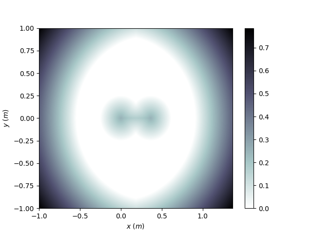
I modeled a few other aspects of this robot. This including making a function that could determine how close a point was to a reachable point by the robot. Unless I see an interest, I will likely not try to explain this as I already have attempted to document this well on the GitHub page. It turned into several if else statements and was frankly a very messy function. Fortunately, after some trial and error, I was able to get it working for any link geometry.

The color represents the distance to a valid point accessible by the robot.

The Next Steps for the Robot

I have only detailed a small portion of the work I did on the robot here. In the next post I’ll focus more on the electronics and hardware used to get the whole thing working. I may even split it into two parts because I made my own motors and will probably write a whole post just about that! Also, I experimented with using the QuickLaTeX plugin in this post and really like how it came out. Hopefully I’ll have an excuse to use it in future posts when more equations pop up, and I would recommend it to others who want LaTeX integrations in their WordPress sites.